Have you ever wondered how computers are able to recognize images? For example, when you see an image like this, you immediately know that it is a cat. But how does the computer know?

From your life experience, you know that a cat typically has sharp ears, round eyes, a triangular nose, and facial hair. The machine wants to figure out important information like that too! At a very high level, the way that image recognition works is that the computer will analyze the image in multiple steps. First, it tries to identify very simple aspects of the images: lines, edges, corners, blobs, etc. Using that information, we build up into slightly, just slightly more complex shapes: squares, circles, triangles. After a few iterations, it starts to recognize high-level features such as eyes, nose, mouth, etc. Finally, by putting all the pieces together, it computes a probability score for this image for each class of objects it could belong to (e.g., cat, dog, bird, etc). As we’ll see later, a layer of connected neurons is responsible for each of those steps and all those layers combine to form a convolutional neural network. A visualization looks something like:

Let’s start building a convolutional neural network (CNN) together. To begin with, the computer sees the image as an array of pixels values. Let’s say the cat image we saw earlier is of size 10x10x3 (where 3 represents the three RGB values). Then the pixel value representation, for one of the 3 RGB color channels, would look something like this:

Then, it scans this entire image a bunch of times, each time looking for one specific feature. Imagine a detective looking for small clues in an image, like sharp corners. He starts by putting his magnifier on the top left corner of the image and slowly scans to the right. When one row is finished, he moves on to the next row. The algorithm we’re going to build will want to do the same thing! It scans the image with a “magnifier”, too.

Now the detective starts scanning! There are a few patterns that the detective is interested in: blobs, circles, colors, and edges. He prepares a few reference objects where each represents a blob, a circle, a color, an edge, etc. He puts the reference object on the image and scans over the image, looking for areas of overlap between the reference and the scanned region.
Mathematically, what the computer is doing is visualized as follows:

In deep learning, this “reference object” is called a filter (also referred to as kernel), and the part of the image that is being compared to is called a receptive field. The amount by which the filter and the receptive field overlap is computed by doing an element-wise multiplication and then summation (dot product). The amount by which the window moves is called a stride. In the above illustration, the filter is of size 4×4 with stride 1. For each position of the filter, it computes a dot product between the filter and the receptive field to compute how much they overlap. For example, if I have a filter that tries to identify round shapes, then my filter might look like this:

Applying this filter on a part of the image:

You see that our “circle filter” aligns very well with this cat’s eye. Suggesting very strongly that there is a circle in this image. Mathematically, it’s no harder than elementary school Math 🙂 It does an element-wise multiplication, and add up all the numbers.
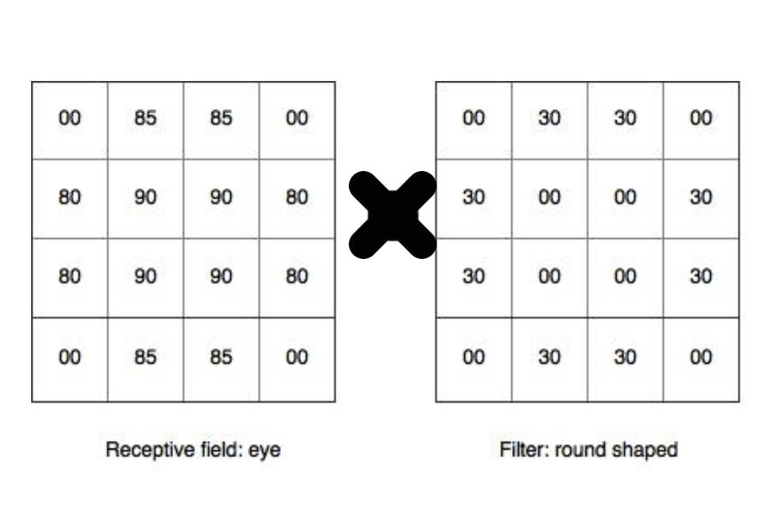
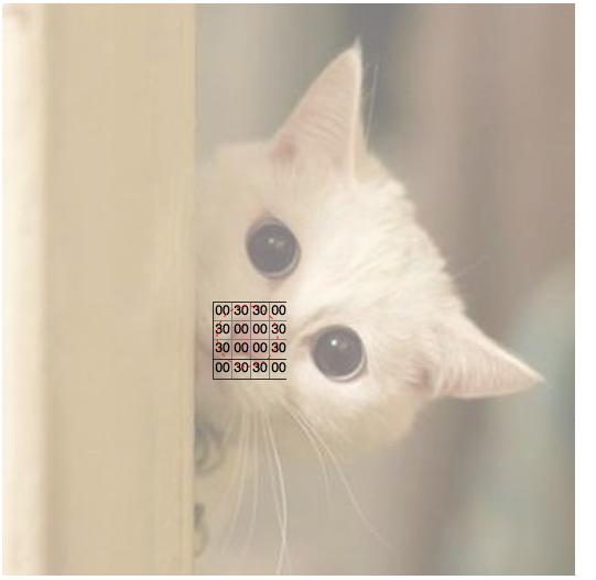
So we’ve got (85*30) + (85*30) + (80*30) + (80*30) + (85*30) + (85*30) + (80*30) + (80*30) = a large number! A large number suggests a high probability that there’s a round shape at this position. In contrast, what happens if the filter scans over a region that does not contain a circle? Like the nose for example:

Doing an element-wise multiplication gives us a matrix of all zero’s, and the sum is also a zero. This suggests that the probability of having a round shape at this location is very low.
Now that we scanned this “round shaped filter” over the entire image, we’re left with a 7×7 array of numbers (because the filter scans over each row and column 7 times). This is called an activation map or feature map. Now, a “round shaped filter” might not be enough to identify anything interesting on its own. We would want a few other filters (e.g., color, blobs, edges) and scan over this image in the same fashion.
Let’s say we have 10 of these filters. Now we’re left with a new “image” of size 7x7x10. So far, we’ve completed one convolutional layer! We usually apply a nonlinear function after each convolutional layer — the purpose of doing this is to increase computational efficiency. Researches and studies have found that ReLU works the best among other nonlinearities and the network can train a lot faster with it. In the ReLU layer, it applies the mathematical function f(x) = max(0, x) to all input values. Namely, it converts all the negative values to 0.
Now, we have a 7x7x10 array of non-negative pixel values that record information about key features in this image. But a lot of this information might not be very useful. Therefore, we reduce the size of the array by subdividing the array into blocks of equal size, and creating a new array consisting of the maximum value in each of these blocks. This method is called max pooling. For example, we can divide up the array on the left side in 2×2 blocks with a stride of two and apply max pooling to get the array on the right side:

So far, we have successfully downsampled the image from 10x10x3 to 7x7x10 and recorded low-level features such as curve, edge, and color. We iterate this process of applying a filter to learn features and downsampling the resulting feature map. Each time we do this, our features become higher and higher level. Before we make a prediction, let’s review our architecture so far:
We started with an image of size 10x10x3. We then fed it into a convolutional layer to learn features about the image. The depth of the output volume is our number of filters (i.e., the number of times we scan over the entire image). We apply ReLU to increase computational efficiency. Then we apply pooling to reduce spatial dimensions. We repeat this process a couple of times before we jump into the final classification step.
Visualized as a neural network, it looks like this:

Recall:
- The input feature map is the representation of the input in pixel values.
- A filter (or kernel) is an array of numbers, and these numbers are called weights. Therefore, a filter is also called a weight vector. This weight vector is the same when we slide over the entire image — that is so called weight sharing.
- A neuron receives some inputs, performs a dot product and optionally follows it with a non-linearity. As per our example, the neurons on the conv layer take the input feature map as an input, computes dot product with the filter (to find out how much they overlap), and follows with ReLU to increase computational efficiency.
- The pooling layer reduces spatial dimension
Got it? Now, let’s make a prediction!
The last layer is a fully-connected (FC) layer. This means that each neuron in this fully connected layer is connected to all neurons in the previous layer. In the FC layer, the input 2D arrays are flattened into a 1D array, and each value gets a vote on which class it might belong to. Some values get larger votes because they think they match some classes better. These votes are expressed as weights. You can think of this process as an election. In practice, multiple FC layers are used where each intermediate FC layer can vote on “hidden” categories, which lets the network learn more sophisticated combinations of features and thus leading to better predictions.
As the figure illustrates, an array of probabilities to each class is computed after the FC layer:

In this example, we see that the probability that the input image is a bird is 0.98, which ranks the highest. Therefore, we predict that it’s a bird! It’s amazing, isn’t it?

Wait a second. It sounds like a cool story, but where do the features come from? How do we find the weights in our FC layers for the election?
That comes to the training part of the network. Like any other typical supervised learning problems, we want to minimize the loss between predicted label and the actual label. We initialize random weights, forward pass the training images with those weights through the whole network, calculate the loss function, perform backward propagation to determine which weights contributed most to the loss, and perform weight update so that loss will decrease in the next iteration. We repeat this training iteration many times. In the end when the model converges, the model has learned the weights and hopefully is ready for testing.
Wait a second. Is it really ready for testing yet? How do we know how many layers, how many features to use in each conv layer, what are the filter sizes in each conv and pooling layer, how many hidden neurons for each extra FC layer, or what is the value for strides? Here comes to the play of hyperparameter tuning. Unfortunately, hyperparameter tuning is more of an art than science. There is no standard for this. Researchers tend to tune them from experience and community knowledge. The reason is that the network largely depends on the type of data you use. Typical hyperparameter tuning techniques include grid search, random search, hand-tuning, and Bayesian optimization. After you’ve found your optimized set of hyperparameters, you are ready to go!

Now, let’s wrap up and take a look at the overall architecture we have described so far:
repeat [conv -> pool] for n times -> FC layer -> prediction
This is the generic architecture. If we specifically have an architecture which consists of 8 layers and looks like this:
conv1 -> pool1 -> conv2 -> pool2 -> conv3 -> conv4 -> conv5 -> pool3 -> fc6 -> fc7 -> fc8
Then we have just described a famous model called AlexNet! AlexNet, released by Alex Krizhevsky, won the 2012 ImageNet Large Scale Visual Recognition Challenge (ILSVRC) and beat the second place by a significant margin. AlexNet started a deep learning revolution. It was a major milestone in the history of deep learning.
In 2014, a newer model with smaller filters and deeper networks came out, and it was VGG. It was the 2nd place in the ILSVRC that year. Instead of 8 layers like in AlexNet, VGG used 16 layers. It entered the ILSVRC competition, and it proved that the depth of the network is a critical component for good performance. The pain point, however, is that VGG has 140 million parameters, which costs a lot of memory and is extremely slow to train. It is currently the most preferred model in the industry for feature extractions. The winner, GoogLeNet, drastically reduced the number of parameters by implementing something called an inception module and improved with computational efficiency. In 2015, the residual network (ResNet) won the ILSVRC competition. It was so-called “revolution of depth”. It featured skip connections and a heavy batch normalization. In 2016, a newer model ResNeXt pushed ResNet to a next level. I encourage everyone who’s interested in deep learning to read their papers to learn about the details!
That’s it for this blog post — hope you enjoyed the material and got a good intuition of what’s happening behind the scenes! Feel free to leave in the comments below if you have nay questions 🙂
Disclaimer: details of the training process and hyperparameter tuning process are omitted because they are beyond the scope of this blog post. Special thanks to Rudi Chen for reading over and reviewing this blog post.


Leave a comment